I. Definition
Image noise refers to the unintended interference superimposed on the target signal during image acquisition, transmission, or processing. Its external manifestation is the random fluctuation of pixel luminance or chrominance (e.g., graininess, color mottling, irregular spots, etc.). Noise directly affects the image signal-to-noise ratio (SNR) and visual quality, and is a core factor limiting the performance of metrics such as imaging system sharpness (MTF) and dynamic range (DR).

Figure 1: Visual examples of typical noise types (from left to right: Gaussian noise, Poisson noise, salt-and-pepper noise, uniform noise, and periodic noise, intuitively showing the different spatial fluctuation patterns of image noise)

II. Categories and Characteristics of Noise
Based on their manifestation in the “temporal” and “spatial” dimensions, image sensor noise can be divided into two main categories: temporal noise and spatial noise. Different types of noise exhibit significant differences in their sources, statistical distributions (PDF), and power spectral distributions (PSD).

General notes:

• PDF (Probability Density Function): Describes the probability distribution of noise amplitude.
• PSD (Power Spectral Density): Describes the distribution of noise power across different frequencies.
• White noise: Refers to a type of noise whose power is uniformly distributed across the entire frequency range; it is a typical type of noise in the frequency domain.

2.1 Temporal Noise
Noise that varies over time, where the value of the same pixel differs across different frames. It mainly originates from processes such as photoelectric conversion, charge transfer, and circuit readout.

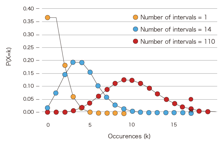
2.1.1 Photon Shot Noise
Source: Statistical fluctuations of incident photons during photoelectric conversion.
PDF: Poisson distribution, approaching a Gaussian distribution at high light intensities.

Figure 2: Photon shot noise distribution under different light intensities (light intensity from low to high (orange → red), the statistical characteristics of shot noise smoothly transition from a Poisson distribution to a Gaussian distribution) [1]

PSD: White noise, with a flat power spectral density across the entire frequency band.
Characteristics: The noise intensity is proportional to the square root of the number of incident photons, based on: $\sigma_{\text{signal}} = \sqrt{N_{\text{signal}}}$

2.1.2 Dark Current Noise
Source: Electronic noise generated by thermal excitation inside the sensor under dark conditions.
PDF: Poisson distribution.
PSD: White noise, with a flat power spectral density.
Characteristics:
Dark current increases exponentially with temperature, based on: $I_{\text{dark}} \propto A \cdot T^3 e^{-\frac{E_g}{kT}}$
$I_{\text{dark}}$: dark current intensity; $T$: absolute temperature (unit: K); $E_g$: bandgap of the semiconductor material (unit: eV); $k$: Boltzmann constant; $A$: proportionality constant related to the material and structure.

Noise increases with the square root of the integration time, based on the standard deviation formula: $\sigma_{\text{dark}} = \sqrt{N_{\text{dark}}}$
$\sigma_{\text{dark}}$: standard deviation of dark current noise; $N_{\text{dark}}$: number of dark charges generated during the integration time.

2.1.3 Read Noise
Refers to the random background noise introduced by the pixel readout circuit and amplifier, including KTC reset noise, thermal noise, 1/f flicker noise, and RTS noise (random telegraph noise) caused by trap effects, etc.
KTC Reset Noise
Source: Voltage fluctuations during the pixel reset process.
PDF: Gaussian distribution.

Figure 3: Probability density distribution (PDF) of KTC reset noise under different pixel capacitances

PSD: White noise, with noise power uniformly and consistently distributed across the entire frequency band.
Characteristics:
The noise is proportional to the square root of temperature and inversely proportional to the square root of capacitance, based on the formula: $V_{\text{KTC}} = \sqrt{\frac{kT}{C}}$
k: Boltzmann constant, T: absolute temperature, C: capacitance value.

Thermal Noise (Johnson Noise)
Source: Full-band random noise caused by the irregular thermal motion of electrons in the circuit.
PDF: Gaussian distribution.
PSD: White noise.
Characteristics: Positively correlated with resistance, temperature, and bandwidth, based on the formula: $V_{\text{thermal}} = \sqrt{4kTRB}$.
$V_{\text{thermal}}$: RMS thermal noise voltage; k: Boltzmann constant; T: absolute temperature (unit: K); R: resistance value (unit: Ω); B: signal bandwidth (unit: Hz).

1/f Flicker Noise
Source: Low-frequency continuous fluctuation noise caused by defects at the device interface.
PDF: Gaussian distribution.
PSD: Significant in the low-frequency band, with power spectral density inversely proportional to frequency (satisfying $S_V(f) \propto \frac{1}{f^\gamma}$).

Figure 4: Comparison of spectral characteristics between 1/f flicker noise and white noise [2]

Characteristics: Exhibits a power-law spectrum with strong low-frequency components and weak high-frequency components, manifesting as slow fluctuations in the time domain.

RTS Random Telegraph Noise
Source: Discrete jump-type noise caused by a few single traps at the MOS transistor interface.
PDF: Bimodal discrete distribution.
PSD: Lorentzian spectrum, decaying as 1/f2 in the high-frequency band.

2.1.4 Quantization Noise
Source: Rounding error noise caused by the limited bit precision of the ADC.
PDF: Uniform distribution.
PSD: White noise, with a flat power spectrum.
Characteristics: Only related to the ADC bit depth; the higher the bit depth, the lower the noise.

2.2 Spatial Noise (Fixed-Pattern Noise, FPN)
Does not vary with time and is caused by differences in the manufacturing process, including: DSNU (Dark Signal Non-Uniformity) and PRNU (Photo Response Non-Uniformity).
DSNU (Dark Signal Non-Uniformity): Originates from the inconsistency in the dark current generation rate among pixels, manifesting as a fixed offset in the pixel background noise under completely dark conditions.
PRNU (Photo Response Non-Uniformity): Originates from slight differences in photoelectric conversion efficiency among pixels, manifesting as spatial fluctuations in pixel photosensitivity under uniform illumination.

III. Noise Evaluation Metrics
Quantitative evaluation of noise typically employs metrics such as RMS (Root Mean Square), SNR (Signal-to-Noise Ratio), and ISO 15739 Visual Noise, among which visual noise is the only evaluation metric that incorporates human visual perception.

Visual Noise
Visual Noise is based on the ISO 15739 standard, which weights the noise spectrum using a human visual system (HVS) model and viewing conditions (viewing distance, display resolution, ambient lighting) to estimate the actual noise intensity perceived by the human eye.
Core difference from Signal-to-Noise Ratio (SNR): SNR measures the total amount of noise, incorporating all noise into the measurement regardless of whether it is visible to the human eye, whereas visual noise is evaluated based on the visibility of the noise, and invisible noise is not included in the measurement.
When the physical noise intensity (such as SNR) is similar, differences in the spatial frequency distribution of the noise will also lead to differences in the visual noise perceived by the human eye. This difference stems from the varying sensitivity of the human eye to noise at different frequencies. Specifically, based on the Contrast Sensitivity Function (CSF), the human eye has lower sensitivity and a weaker CSF response to high-frequency noise, but higher sensitivity and a stronger CSF response to low-frequency noise. As shown in the figure below, the 1x noise image appears as fine high-frequency grain, while the 4x noise image presents as a low-frequency checkerboard pattern. Even if the total physical noise is similar, the visual noise value of the 4x noise image is much higher than that of the 1x noise image.

1x, 2x, 4x noise images

CSF curve

Root Mean Square (RMS)
Root Mean Square (RMS) is a statistic that describes the average fluctuation amplitude of data and is widely used in signal processing, engineering, and other fields. In image noise quantification, RMS is the core measurement metric characterizing noise intensity, and its value is equivalent to the sample standard deviation of the signal S from a uniform gray patch, namely: $$\text{RMS Noise} = \sigma(S)$$

Noise power can be directly obtained by squaring the RMS noise: $\text{Noise Power} = (\text{RMS Noise})^2$.

The formula for calculating the standard deviation is: $$\sigma = \sqrt{\frac{\sum_{i=1}^{n}(x_i - \bar{x})^2}{n-1}}$$ where $\sigma$ represents the sample standard deviation; $n$ represents the number of data points; $x_i$ represents the $i$-th data point; and $\bar{x}$ represents the mean of all data points.

In image noise testing, a uniform gray patch is typically selected as the ROI, and its RGB pixel values are converted to the luminance channel Y (the typical calculation formula is Y=0.2125R+0.7154G+0.0721B). The sample standard deviation of this region is then calculated based on the above formula, which yields the RMS noise for the corresponding luminance channel.

Signal-to-Noise Ratio (SNR)
Signal-to-Noise Ratio (SNR) refers to the ratio of the signal mean to the total noise standard deviation, used to evaluate the system's ability to extract valid signals in the presence of noise. A higher SNR indicates lower image noise and clearer details; a lower SNR indicates more obvious noise interference. Its mathematical expression is:
$$SNR = \frac{\mu_{\text{signal}}}{\sigma_{\text{total}}}$$ $\mu_{\text{signal}}$ is the mean of the image signal (average output value DN); $\sigma_{\text{total}}$ is the standard deviation of the total noise.
SNR is commonly expressed in logarithmic form as: $SNR(\text{dB}) = 20\log_{10}\!\left(\frac{\mu}{\sigma}\right)$

IV. Common Noise Reduction Filtering Methods
Images are susceptible to noise interference during generation and transmission, which affects quality and subsequent processing results. Filtering is a common method to suppress noise and improve image clarity. The following introduces four commonly used noise reduction filters: mean filtering, median filtering, Gaussian filtering, and bilateral filtering.
Gaussian Filtering
Centered on the target pixel, it takes the weighted average of the grayscale values of the pixels in a 3×3 neighborhood to update the center pixel. This method can effectively suppress Gaussian noise, causes less loss of image clarity than mean filtering, and provides a more natural smoothing effect. It is a commonly used linear filtering method in image processing.
Mean Filtering
It assigns the average grayscale value of the target pixel and its surrounding pixels to the target pixel. This method is simple to calculate and relatively thorough in noise reduction, but it easily loses image edges and detail information during the noise reduction process.

Median Filtering
It sorts the grayscale values of the target pixel and its surrounding pixels, and takes the median value as the target pixel value. It has a good effect on removing discrete noise such as dead pixels and salt-and-pepper noise, and can better protect edges, but its overall noise reduction effect on continuously distributed noise is average.

Bilateral Filtering
Based on Gaussian filtering, it adds pixel value weights, taking into account both spatial distance and grayscale similarity, to better preserve edges while reducing noise.

Image sources: [1]https://camera.hamamatsu.com/jp/en/learn/technical_information/thechnical_guide/photon_shot_noise/_jcr_content/root/container/container_1525074977/container/image.coreimg.jpeg/1655376117368/s-lsc-te-tg-wpsn-1-en.jpeg
[2]https://upload.wikimedia.org/wikipedia/commons/thumb/f/f6/Fc.png/500px-Fc.png
Gaussian filtering: https://blog.csdn.net/jiandanjinxin/article/details/51281828
Median filtering, mean filtering: https://bioimagebook.github.io/chapters/2-processing/4-filters/filters.html